Adversarial Patches and Autonomous Vehicles
Intro
Imagine a self-driving car passing a strange looking piece of graffiti. All of a sudden, the vehicle fails to respond to a stop sign, and runs into an intersection. That piece of “graffiti” might have been an adversarial attack. In this post, I’ll give you the context for my NC Science and Engineering Fair project, which I later expanded into a research paper (Arxiv) on defending autonomous vehicles against adversarial attacks, and share some of the really fascinating things I’ve learned over the last 2 years.
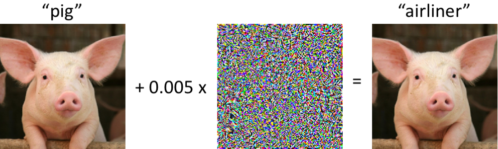
The leftmost image in the diagram above is a perfectly normal photograph, which is correctly classified as a pig by a well-trained ResNet model. By adding a tiny amount of specially generated noise to the image, we get the image on the right. Although the intensity of the noise is so low that the 2 images look the same to a human, the ResNet model now classifies the second image as an airplane! This is called an “adversarial example attack”, or an “adversarial perturbation”.
Adversarial Perturbations
Of course, the vast majority (by which I mean almost all) of the possible perturbations/patterns of random noise don’t cause ML models to make such ridiculous misclassifications. Adversarial perturbations are very carefully designed layers of noise that usually require access to a model’s weights (whitebox access), assumptions about a model’s architecture and differentiability, and a bit of computational power to generate.
FGSM (Fast Gradient Sign Method)
The example I provided above is a targeted attack generated by something called FGSM, but I think it’s a bit easier to first explain how FGSM generates untargeted attacks. A model’s loss on a specific image tells it how well it did on classifying that image. When we take the gradient of the loss function with respect to the model’s parameters, we get “nudges” to the model’s weights that improve the model’s performance on that sample. This is pretty standard stuff in training a model, but something really interesting happens when we take this thinking a little further.
Because almost all modern architectures are fully differentiable, we can take the gradient of the loss with respect to the pixels in the input image, instead of the parameters of the models. This gives us a “nudge” to the pixel values in the image that would encourage the model to classify an image as the ground truth label. As it turns out, this gradient looks almost like random noise to the human eye. And if we multiply this gradient by some very small negative number, we get a nearly imperceptible amount of noise that when added to the original image, causes the model to be less likely to classify the image as the (correct) ground truth label.
This is almost exactly how FGSM works, except that FGSM discards the magnitudes of the gradient and only uses the sign. Because this noise vector is in the exact direction that best causes the model to do worse, it causes the model to make misclassifications even at low intensities.
What I described above is an untargeted attack, since we just generally increase the loss. However, if we replaced the loss function with a specific objective function, our attack becomes targeted. For example, instead of generally wanting the model to perform worse, I might specifically want it to classify an input image as a cat. Then, given model P, I might define the loss as L = -P(“cat”|X). When I take the gradient of this with respect to X, I’ll find the noise vector that maximizes the probability of the model predicting “cat”. We call the sum of the original image and the perturbation an adversarial image. Generally, Xadversarial = X + ɛ * ∇XL(P, X, Y), wher epsilon represents the intensity of the noise.
Adversarial Patches
Luckily for us, adversarial perturbations aren’t a big threat in the real world. Although they can make life harder for models operating on images in a purely digital world (I’m pretty sure Captchas are made more difficult for computers through adversarial perturbations), nobody can force the camera of a self driving car to see precise amounts of low intensity noise everywhere in its field-of-view.
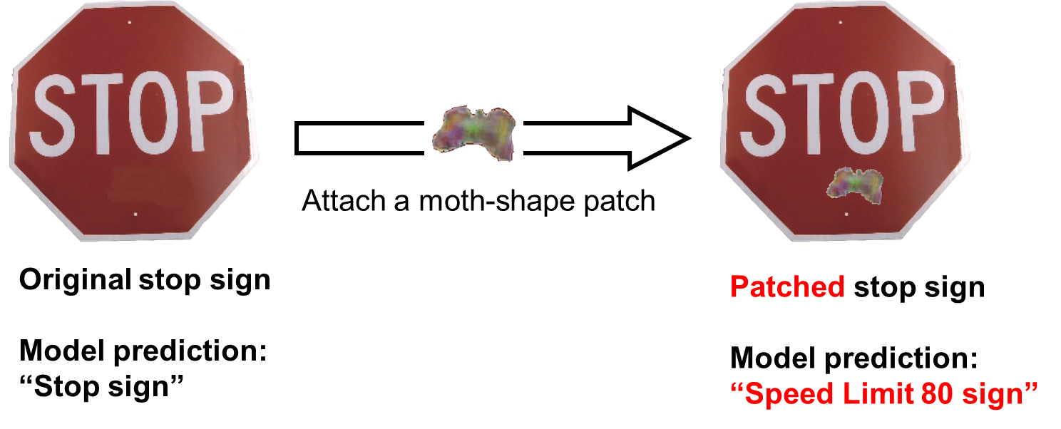
Unfortunately, there’s a more potent attack called an adversarial patch attack that is realizable in the physical world. To solve the issue of natural image noise and lighting breaking perturbations, adversarial patches have no restrictions on the intensity of the perturbation. To solve the issue of being unable to force a camera to see noise across its entire FOV, adversarial patches are designed to only need to cover a small portion of an image. To solve the issue of changing perspective, positions, etc. in the real world, different geometric transformations are sampled throughout the training process of an adversarial patch.
FGSM only took the gradient of the model once (essentially assuming the loss surface was linear). However, because adversairal patches have a much higher intensity and have to work in a much less accomodating environment, they’re trained with Projected Gradient Descent (PGD). We can think of PGD as more or less the same as gradient descent: the gradient is taken many times for many samples, and the patch is updated many times to avoid the errors from a linearization.
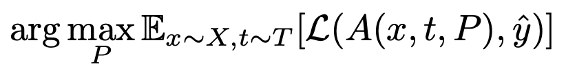
Specifically, PGD is used to solve the above optimization problem, where P represents the patch, T represents the distribution of real world transformations (scaling, changing positions, rotations, perspective changes, etc.), A represents an applier function that superimposes a patch with some applied transformation t onto image x, and y represents the ground truth of x. By maximizing the expectation of the loss across all transformations, we’re able to obtain a patch that works in the real world. Importantly, we can use gradient-based methods to solve this optimization problem as long as the transformations can be represented as transformation matrices (e.g. rotation matrix).
Applying it to Autonomous Vehicles
For an autonomous vehicle to make good decisions, it must have a good representation of the world around it. This comes from its perception pipeline, which extracts relevant objects and features from its camera feed. A crucial stage in this pipeline is object detection, where relevant objects (e.g. pedestrians, other cars, traffic signs) are labeled and localized (a bounding box is drawn around the object).
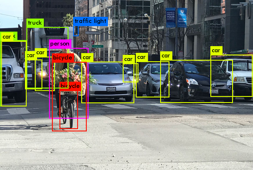
Frequently, a convolutional neural network architecture called “YOLO” is used for object detection. YOLO predicts many bounding boxes (varies by version, I know YOLOv5 predicts 25000+), which are defined by the x, y, w, h of the boxes, the predicted label of the object in the bounding box, and crucially, the confidence of the prediction. Obviously, there aren’t usually 25000+ objects in a scene, which is why most objects with a very low confidence are filtered out.
However, this also provides us with an easy objective to attack. Combining the idea of targeted adversarial attacks with the general objective for adversarial patches, we define the loss to be the confidence vector that the YOLO model outputs. This is the idea behind the “object vanishing adversarial patch”: the adversarial patch is trained to minimize the model’s confidence across all boxes, which means almost all predictions will be filtered out.
This is obviously a huge threat, since it means self-driving cars might fail to detect pedestrians, other vehicles, and important objects on the road. Worse, most defenses against adversarial patches are slow, and aren’t applicable to the rapidly changing environment autonomous vehicles face. These are some of the challenges I try to address in my paper, which you’re hopefully a little more prepared to read.