The Math Behind Asteroid Impact Prediction - Will the Flat-o-Saurs Go Extinct?
65 million years ago, all the dinosaurs were killed by a big asteroid. The Flat-o-saurs are kinda like the dinosaurs, but they live on a 2D planet called plane-et, which exists in a 2D universe. Dr. Bi-ceratops, the 2D cousin of the 3D Triceratops, has set up an asteroid detection and monitoring system to try to avoid his cousin’s tragic fate.
Oh No! Dr. Bi-ceratops has detected an asteroid! In this paper, I’ll explain how Dr. Bi-ceratops’ detection and monitoring system works, and how he can calculate the probability of the newly discovered asteroid hitting plane-et.
To find asteroids that might be a threat, Dr. Bi-ceratops has set up cameras pointed at the night sky. Sophisticated software analyzes the images from these cameras, and flags fast moving objects (which are likely to be asteroids).
Because the cameras only capture an image, they can calculate the angle of the asteroid relative to plane-et, but can’t (easily) find the distance of the asteroid to plane-et (the image has no depth information associated with it.)
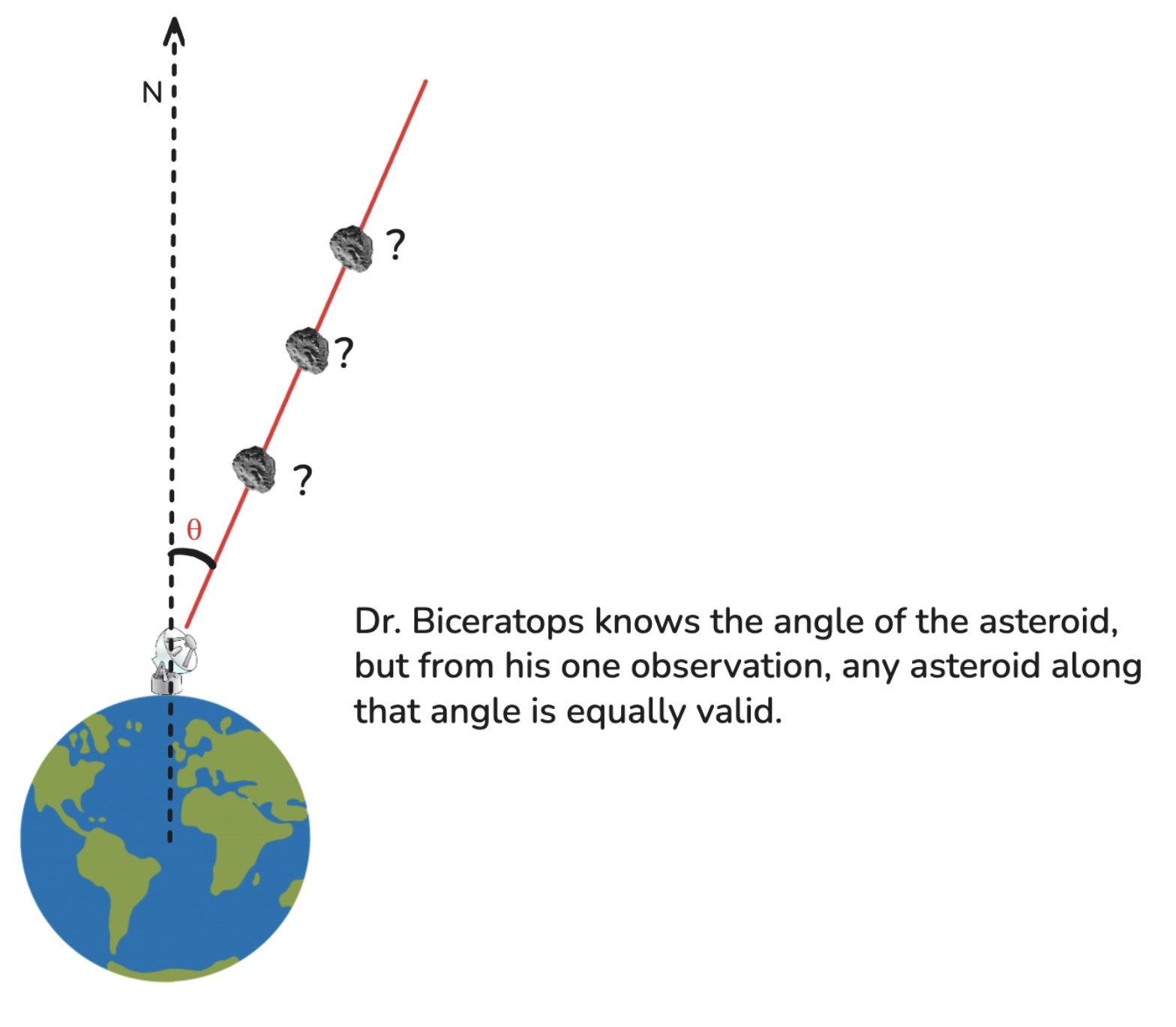
Before Dr. Bi-ceratops can predict whether the asteroid will hit plane-et, he needs more information about the asteroid. To fully describe an asteroid in 2D space, Dr. Bi-ceratops needs its x and y coordinates, as well as its x and y velocities. From his one observation, all Dr. Bi-ceratops knows is θ. He knows that x and y are related to θ by x = r * cos(θ) and y = r * sin(θ), where r is the distance from plane-et to the asteroid. Unfortunately, he still doesn’t know r, vx, or vy.
Luckily, Dr. Bi-ceratops can make multiple observations!
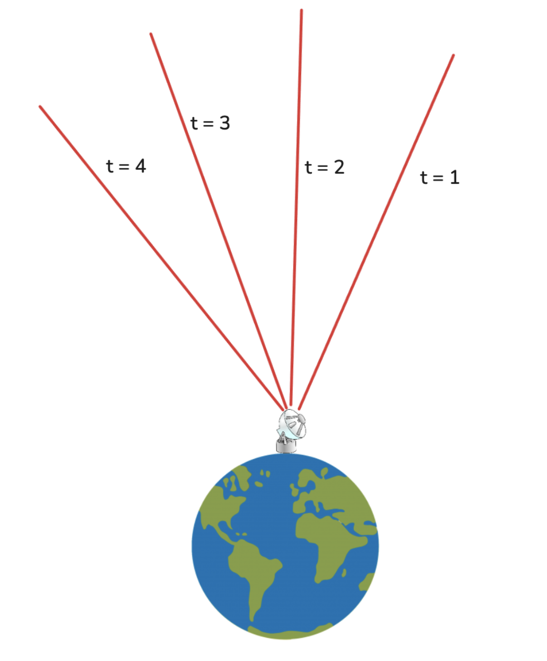
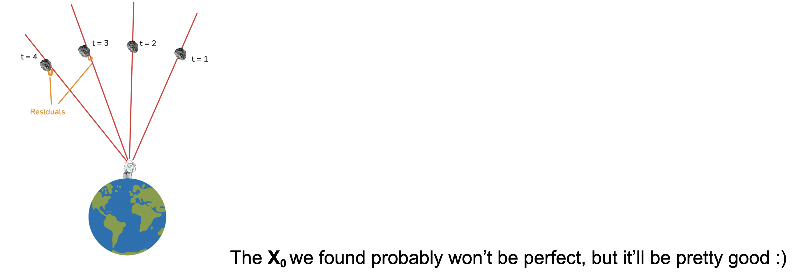
How can he use these multiple observations to help him find the unknown r, vx, and vy? He can do what I do on every math test: guess start with an estimate, and refine it until the estimated asteroid is consistent with every observation.
Let’s generate an asteroid with random r, vx, and vy at t=1, and simulate its motion according to Newton’s laws of motion.
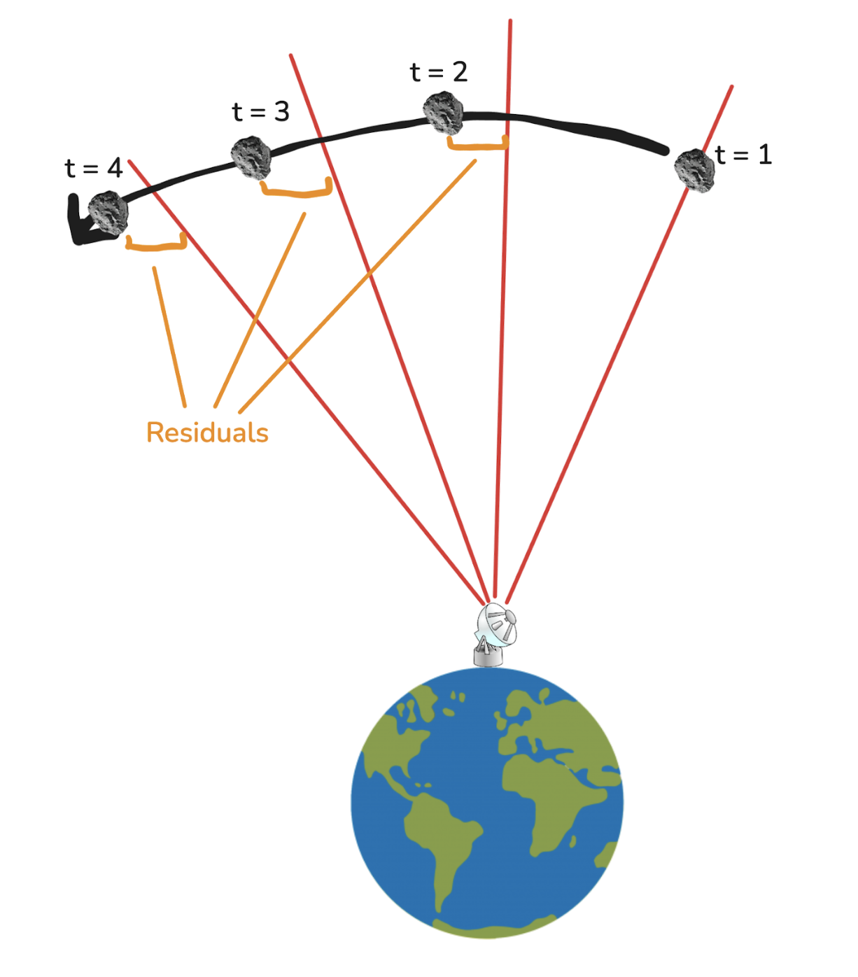
Hmm…this specific combination of r, vx, and vy is not consistent with all the observations (it has large residuals). This means we probably haven’t found the values that best characterize the asteroid. However, if we find some combination of r, vx, and vy that has small residuals, we’ll know we’ve found a good characterization of the asteroid.
Formally, we want to find the combination of r0, vx_0, vy_0 which when propagated forward in time using Newton’s laws of motion, minimize the weighted squared residuals relative to all observations.
Let’s define the following cost function Q:
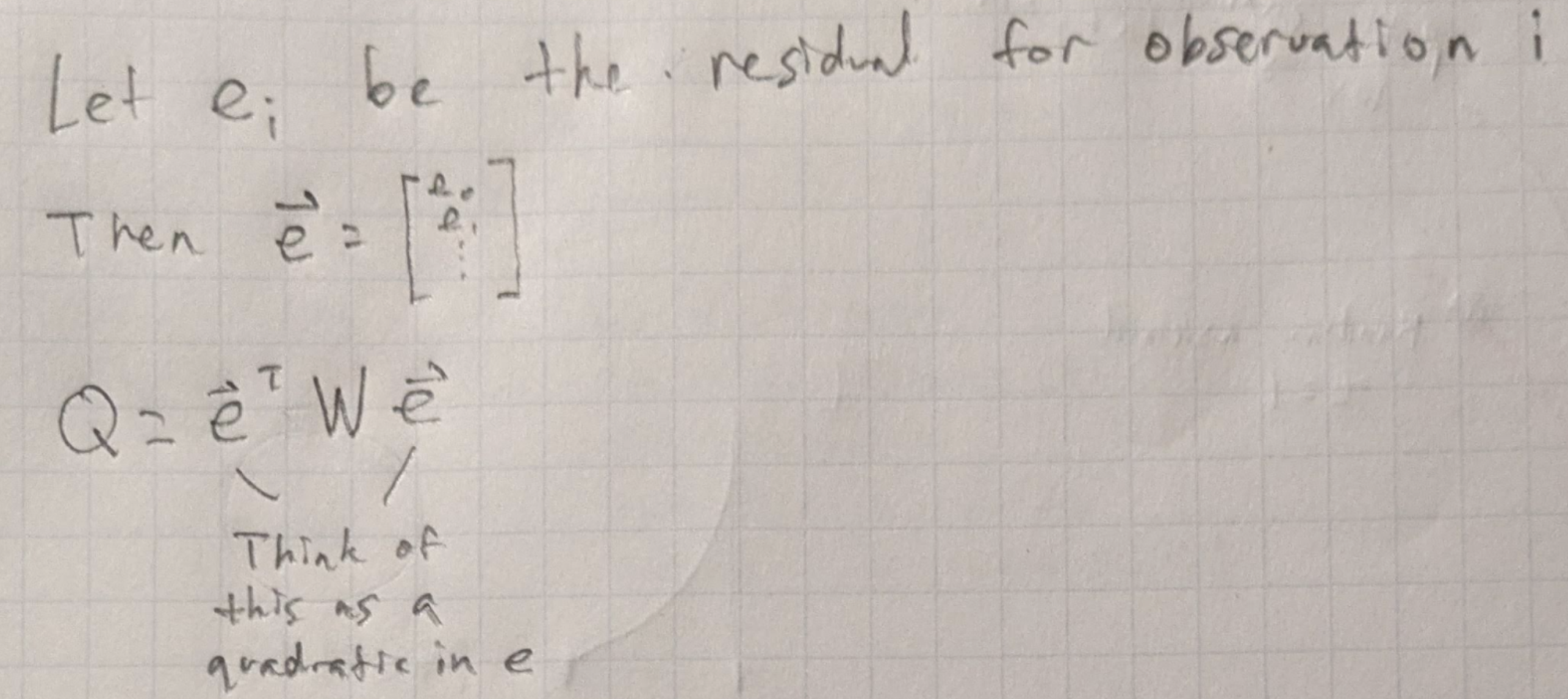
As you can see, Q is a quadratic function of the residuals, although the form is a bit funky cause e is a vector. W is a weighting matrix, since some residuals may be less important than others to minimize. If all residuals are weighted the same, W would be the identity matrix.
So, Dr. Bi-ceratops needs to find the initial state of the asteroid which when propagated forward in time, minimizes Q. How can Q be minimized? Harkening back to Calculus 101, Dr. Bi-ceratops vaguely remembers that a minima of a function occurs when its derivative (or in this case, gradient) is 0 (definition of a kritikal point!) P.S.: Typically, we wouldn’t know if the critical point was a min or max, but it turns out this cost function is highly convex in practice.
Let’s define the initial state of the asteroid as X0, where X0 = [r0, vx_0, vy_0]. Note that X is the entire characterization of the asteroid, not just its x coordinate.
Formally, we need to find the value of X0 where ∂Q/∂X0 = 0. To do this, we’ll start with an initial random (and probably bad) estimate of X0. Then, we’ll refine X0 by repeatedly changing it by some small δx until we’ve found the X0 where ∂Q/∂X0 = 0.
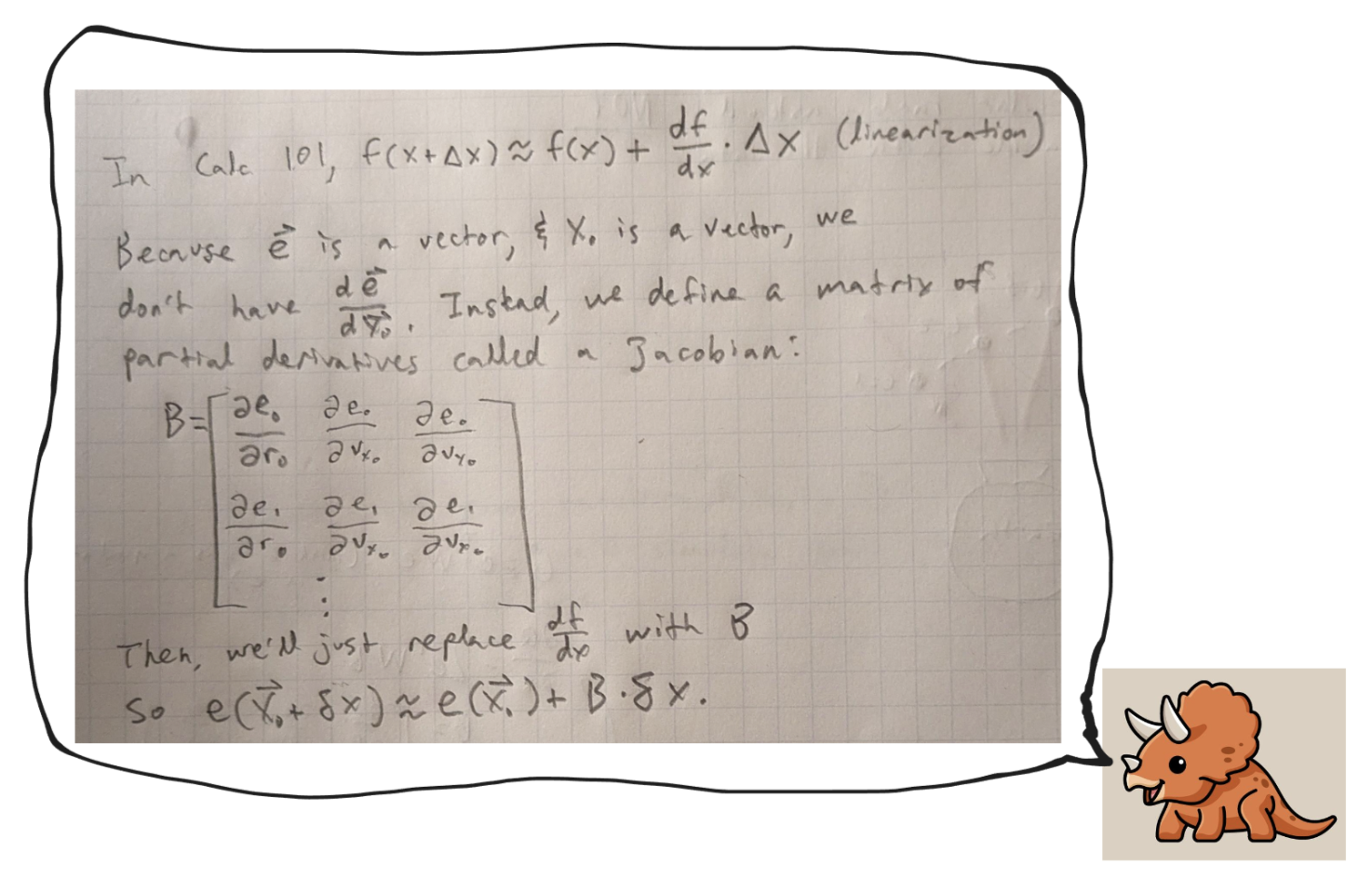
Now, how do we find the right δx to change X0 by? Let’s examine what happens to the residuals when we change X0 by some small δx. We assume e(X0) (remember, e represents our residuals) is locally linear. Then, e(X0 + δx) ≈ e(X0) + B * δx, where B is the Jacobian ∂Q/∂X0. If this is a bit confuzzling, scroll down and Dr. Bi-ceratops will explain it better.
This in turn means that Q(X0 + δx) = e(X0 + δx)T * W * e(X0 + δx)
= eT*W*e + 2δxT*BT*W* e + δxT*BT*W*B*δx after expansion.
Whew! That expansion took me like 40 minutes. But it was worth it, because if you look closely at the expanded expression, we see that the change in Q with respect to a small change in X0 (δx) is:
2 * BT * W * e + BT * W * B * δx
Wait a second! A small change in Q with respect to a small change in X0?? That’s ∂Q/∂X0!
Therefore:
2 * BT * W * e + BT * W * B * δx = 0
which rearranges to:
δx = -C-1 * BT * W * e
where C = BT * W * B.
Note that C is also the second-order partial derivatives of Q (C is the Hessian of Q).
So it turns out that:
δx = -C-1 * BT * W * e.
This means that by updating X0 by -C-1 * BT * W * e repeatedly, we’ll eventually refine our characterization of the asteroid into something that’s compatible with all observations!
So we’ve found a X0 that is the best characterization of the asteroid. However, because there’s some uncertainty in our measurements, and because the X0 we found still doesn’t lead to a path that fits perfectly with all observations, X0 is actually a multivariate probability distribution centered at the best singular X0 value we found. From now on, I’ll use X0 to represent the probability distribution, and Xbest to represent the singular value we found previously.
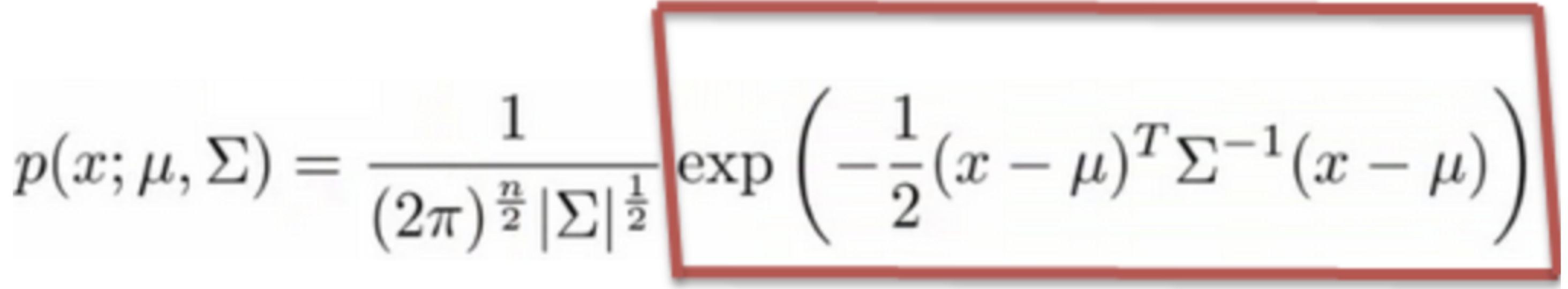
Let’s assume X0 is Gaussian. A multivariate Gaussian takes the form:
 Σ represents the covariance matrix of the distribution (this is like standard deviation but in more dimensions).
We already know μ is Xbest, so what we need to find now is the covariance Σ.
Intuitively, some X ~ X0 with a high cost (Q) has a lower probability than a X with a low cost, since it is less compatible with the observations.
We’ll formalize this idea as Q(X) ~ -log(P(X)) + Constant. This means that a X with a high cost has a probability approaching 0, and a X with a low cost has a probability approaching 1.
Rearranging, P(X) ~ exp(-Q(X)).
Now, how do we calculate Q(X)? Let’s do a second-order Taylor series expansion around Q(Xbest): Q(X) ≈ Q(Xbest) + ∇Q(Xbest)T * (X - Xbest) + ½ * (X - Xbest)T * H * (X - Xbest), where H is the Hessian of Q(X) (the Hessian is the second-order partial derivatives).
Now, recall that at Xbest, the gradient is 0 (Xbest is a minima, which means it’s a critical point).
This means ∇Q(Xbest) is 0.
Also recall that we found that C was the Hessian of Q, which means we can simplify our Taylor series expansion to:
Q(X) ≈ Q(Xbest) + ½ * (X - Xbest)T * C * (X - Xbest)
Here’s the most satisfying part of Dr. Bi-ceratop’s system (in my opinion).
Plugging in the Taylor series expansion for Q(X) into
P(X) ~ exp(-Q(X))
gives:
P(X) ~ exp(-½ * (X - Xbest)T * C * (X - Xbest))
That’s exactly the form of the red boxed thing in the definition of a multivariate Gaussian (recall Xbest is the mean)!
This means that we already have the covariance matrix calculated:
it’s just the inverse of the final value of C we calculated when we found Xbest!
So basically for free, we have the probability distribution of the initial location and velocity of the asteroid based on just angle observations. Plotting just the location (x, y), we get a distribution like the following:
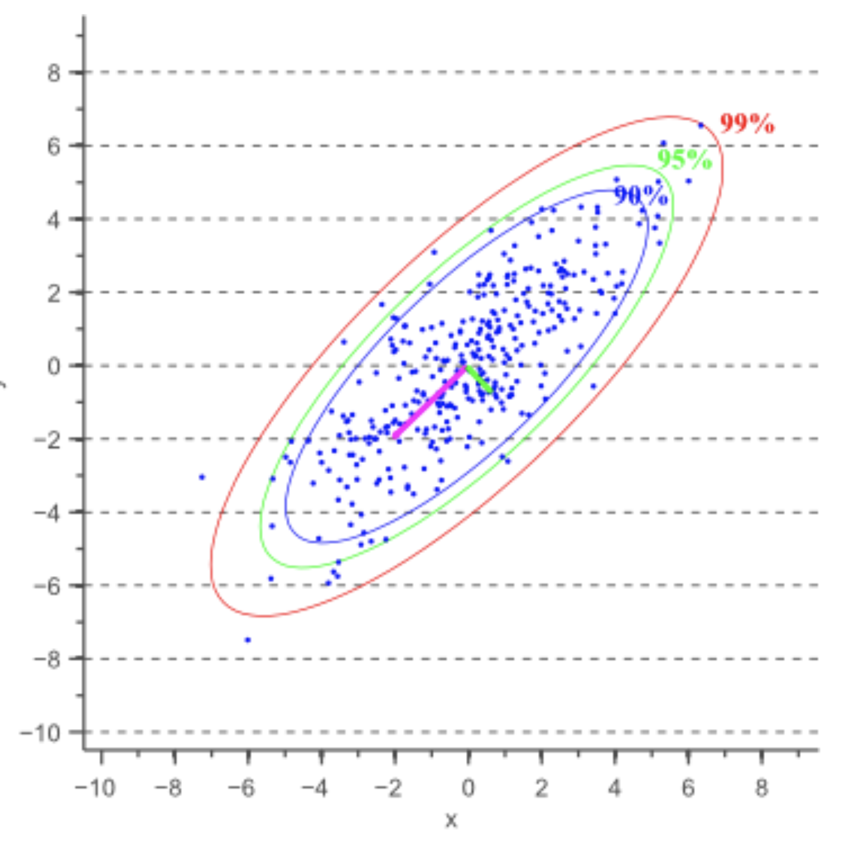
If Dr. Bi-ceratops were a 4 dimensional creature instead of a 2 dimensional creature, he’d be able to see that the actual distribution looks like a 4D hyperellipsoid describing the uncertainty in x, y, vx, and vy!
Now that the asteroid is pinpointed, it’s pretty easy*** to calculate the probability of impact with plane-et. Just sample a bunch of asteroids from the probability distribution, simulate their paths using Newton’s laws of motion, and check if they collide with plane-et - and boom ☄️ - we’re done!

*** What I described for calculating probabilities is really slow cause you have to sample a lot of asteroids - there are much better and faster ways that I would write about but the flat-o-saurs are after me and I don’t have tim-