Algorithmic Gerrymandering Pt. 2: Gerrymandering the Lattice Model

The Foundations

In the previous article, we created a lattice model to represent the map we have to gerrymander, where all the tiles belong to one giant region. Now, we have to create the set of gerrymandered districts. A district in our case is just a list containing all the tiles in it, filling some constraints. It must be continuous - meaning that every tile in it must be reachable from any other tile in it without crossing into a different district, and all districts must have relatively similar populations.
To actually generate these districts, we’ll start with a random(ish) starting district set and slowly make the map more gerrymandered with simulated annealing.

Voronoi tessellations

To generate a gerrymandered set of districts, we have to come up with an initial set of districts to build off of. Our initial districting should fill our constraints of contiguity (since this is something hard to slowly optimize for) but doesn’t need to be gerrymandered or have equal population. To do this, we use a technique called Voronoi tessellations.

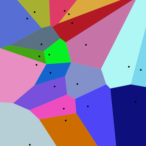
To create a Voronoi tessellation, we drop n random points known as generators onto our grid. Each of these points will be a starting point for a district. We then loop across each cell in our lattice, computing the distance of that cell from each of the n generators. That cell is then assigned to the district of the generator it’s closest to. In essence, we are creating n polygons such that every point in any given polygon is closer to its generator point than the generator point of any other polygon. Our algorithm for computing Voronoi tessellations with it’s O(n²) time complexity is not the most efficient - Steven Fortune’s plane sweep method can compute the same tessellation in O(nlogn) time - but it is the simplest and most intuitive algorithm.



Voronoi tessellations have many other applications. For example, if we generate a Voronoi tessellation on a town with fire stations as the initial points, we know that the closest fire station to any given fire is the one in the same cell of the Voronoi tessellation as the fire. Voronoi tessellations are also often found in nature, such as honeycomb or the wings of a dragonfly.

Simulated Annealing

To actually gerrymander the initial set of districts we’ve generated, we’ll use an algorithm called simulated annealing.
Simulated annealing is used to find optima of a function. Simulated annealing in computer science is based on the annealing process in metalworking. In annealing, metals are heated up to a very hot temperature, so that the excited particles move around before cooling back down. The hope is that in the random jostling, the particles will be more likely to settle into more stable locations and therefore form a stronger material. In simulated annealing, we start with a random solution and a very high “temperature”, making lots of random adjustments to the initial solution and generally accepting better solutions to iterate further upon. However,we’ll also occasionally accept inferior solutions to explore the state space and avoid local optima - the higher the “temperature”, the more likely we are to accept an inferior solution. Later on in the optimization process, we’ll drop the “temperature” to finetune a good solution. The temperature should balance exploration with exploitation - the algorithm must be willing enough to accept a worse solution to explore enough of the function to find the approximate location of the global optimum, but also likely enough to choose to stick with the better solution to converge on the exact location with exploitation. Doing when round of this random change and evaluation is called an iteration. To find a good solution, often tens of thousands of iterations are needed.

Putting it all together

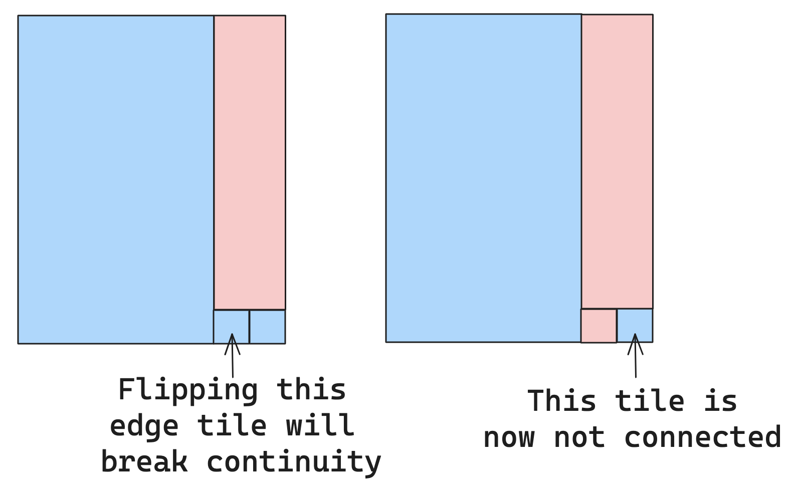
To generate the initial “random solution” that simulated annealing needs to start with, we create a voronoi tessellation to form the initial districts. Simulated annealing then randomly flips tiles to different districts to create new district sets. Because districts need to remain continuous, we can only flip edge tiles (tiles bordering another district). Every step of the simulated anneal, we flip one of these edge tiles from the district it’s currently in to the district it’s bordering. Before we do anything with the new solution, we’ll need to make sure that all districts remain continuous after removing the tile (even flipping an edge tile can break continuity).


Then, we use some mystery evaluation function (to be explained later) to determine whether the new district set with the single tile flipped is better or worse than the previous one. If it’s better, we’ll set the new solution as the main solution we’ll iterate on in the future. If it’s worse, we’ll use the temperature to determine whether to keep it or not by generating a random number from 0 to 1 - if the random number is less than the temperature, we’ll use the new solution (the temperature will be a decimal representing the probability of accepting an inferior solution). This way, we occasionally accept an inferior solution to avoid getting stuck in a local optimum.

The Mystery Evaluation Function

We need to optimize for three things to create a valid gerrymander - the map needs to not only strongly favor one party but also ensure that all districts have similar populations and are fairly compact. Optimizing for similar populations is easy to do - all we need to do is calculate the standard deviation of the total populations of each district (we’ll find the total populations of each district by summing the population attributes of each tile in that district). Optimizing for compactness is significantly harder. The simplest metric for compactness is the perimeter-area ratio. A shape with a large perimeter but low area is probably not very compact - think of a very long rectangle. On the contrary, a shape with a large area but small perimeter is probably very compact - think of a square. However, as we’ll find out later, this method does not do a great job of ensuring that districts are compact. To optimize the map to favor one party, we could simulate an election with the new district set and see if the party we’re favoring wins. However, simulated annealing needs to be able to measure slow incremental progress - remember, we are only making tiny changes. Checking the number of districts our favored party wins is the opposite of slow, constant progress - instead, progress is made in big jumps of winning an extra district. Therefore, because this method can’t diffrentiate between a slightly better and slightly worse districting, our simulated annealing algorithm will just randomly stumble around, unable to make incremental progress towards a good solution. Instead, we’ll remember that the two main methods of gerrymandering are cracking and packing, as explained in the previous article. Based on the findings of the paper “Optimal Gerrymandering: Sometimes Pack, but Never Crack”, we’re only going to pack. Recall that packing sets out one or two districts for “packing”, which are filled with an excess of opposing voters. Every other district is fairly close but gives a small advantage to the gerrymandering party. To replicate this behavior, we’ll create a target margin of victory for each district, giving the packing districts a target value strongly in favor for the opposing party, while giving every other district a target value slightly in favor of the gerrymandering party. For example, targets favoring blue (negative) if 5 districts were needed would look something like [-0.05, -0.05, -0.05, -0.05, 0.20]. Notice how blue wins 4 districts by a small margin (0.05) while red only wins one, but by a margin equal to the margins of all the blue districts combined (0.20). Then, we can calculate the average difference between the target and actual margins of victory for each district. This does allow us to measure small amounts of progress - even if we don’t win a district, if we take a small step towards what our target margin is, the standard deviation will drop by a little bit. By creating a weighted sum of these 3 values, we can return a evaluation for any given set of districts. A higher evaluation will mean a worse set of districts, because that means it has a higher deviation in population between districts, more perimeter-area, and/or more difference from the target margins of victory.

Results

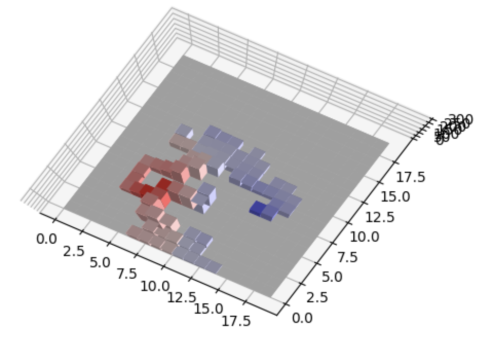
The example below takes a very slightly blue overall map and gerrymanders it such that 4 districts go to red and only 1 goes to blue. The targets were [0.05, 0.05, 0.05, 0.05, -0.20] and 10000 iterations were run.
The overall map is shown below.
The districts that red wins are by tiny margins. In fact, they almost look equal. 2 of the 4 districts red won are displayed below.
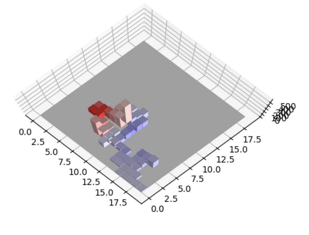
In contrast, the 1 district blue wins is obviously overwhelmingly blue.
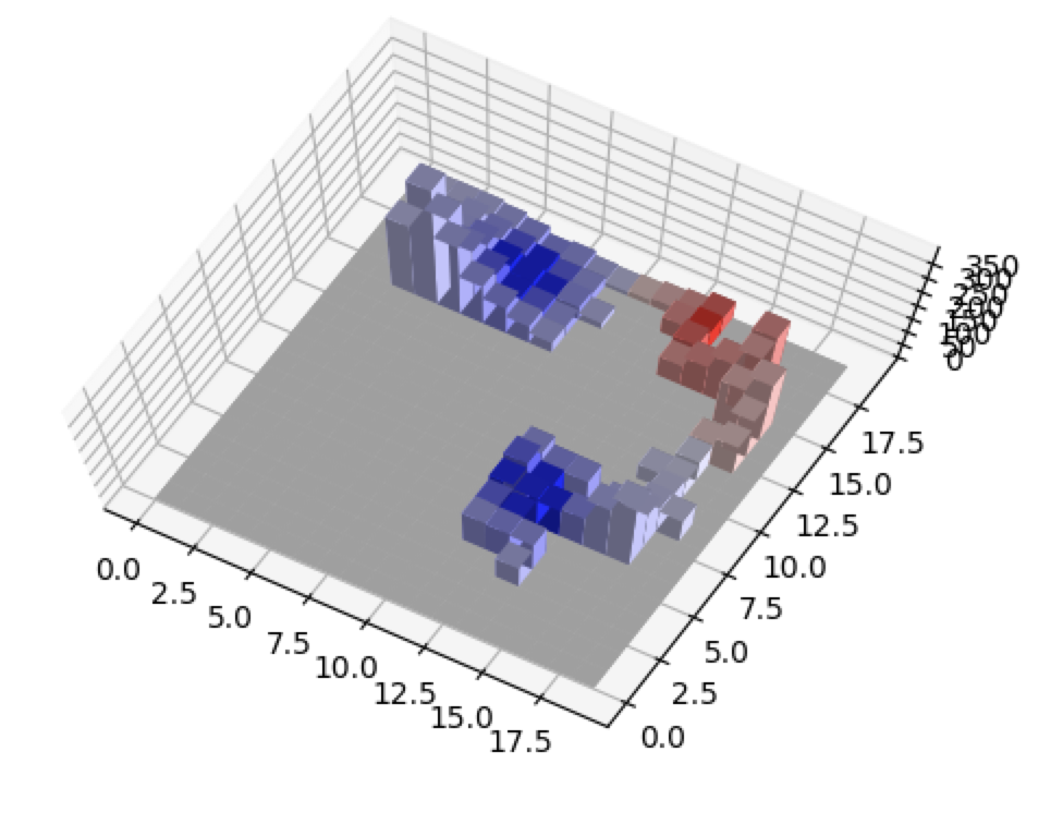
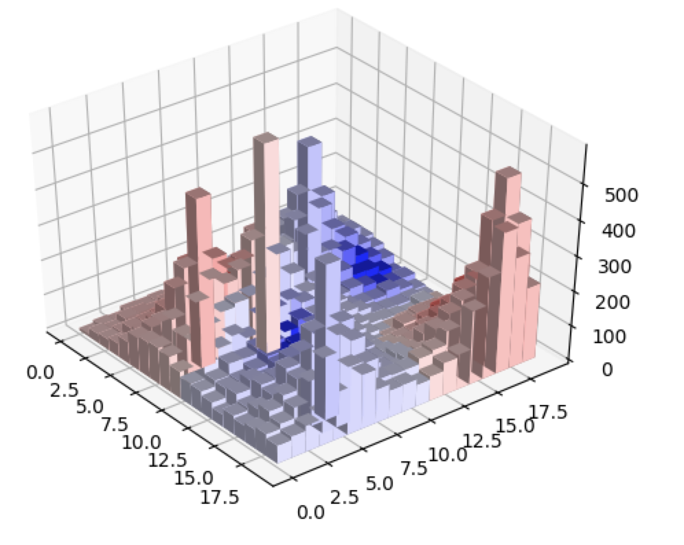
The algorithm did exactly what we wanted it to - the blue district is packed while the red districts are only slight wins by red. Also notice how the populations of each district are relatively close - The total heights of all the bars in each district are pretty similar.
The evaluation of the initial set of districts was over 40000. By the end of the the simulated anneal, the evaluation was less than 4000, showing us that the simulated anneal did its job.

Optimizations and Future Work

Optimizations

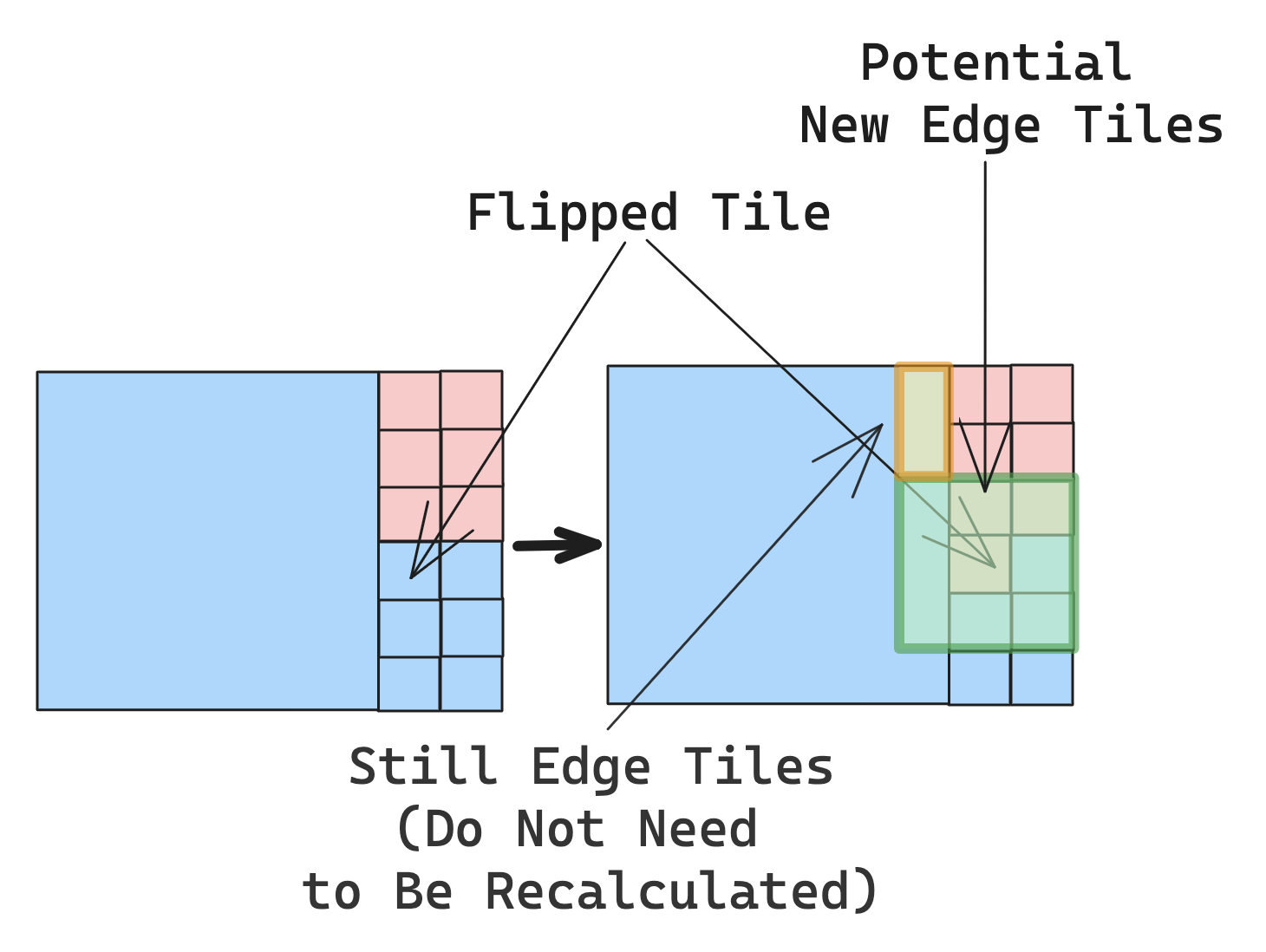
Generating that list of edge tiles to randomly flip is an extremely time consuming process that must be run thousands of times. Therefore, it’s important not to perform redundant calculations. Instead of regenerating the entire list of edge tiles every iteration, we notice that since we’re only flipping one tile at a time, only the 8 tiles immediatley surrounding the flipped tile can possibly be new edge tiles. Every other edge tile in the previously generated list will remain an edge tile. Therefore, we only need to recheck the 8 surrounding tiles to see if they remain edge tiles or if they are new edge tiles.


Essentially the same optimization can be applied to calculating the standard deviation in population between districts. To find the standard deviation of populations for each district, we first need to actually find the population in that district. Because districts are composed of tiles which each have a population element, the total population can be found by summing the population of every tile. However, because districts can be composed of dozens of tiles, its also quite slow to recalculate the total population for every single district (even ones that didn’t gain or lose a tile) by summing up every single tile in that district (even if that tile didn’t change districts). Instead, we can simply calculate the population in every district once and store that. Then, every time a tile is flipped, we simply subtract the population of that tile from the population of the district it was in, and add the population of that tile to the district it was added to, avoiding hundreds of wasteful operations.

Future Improvements

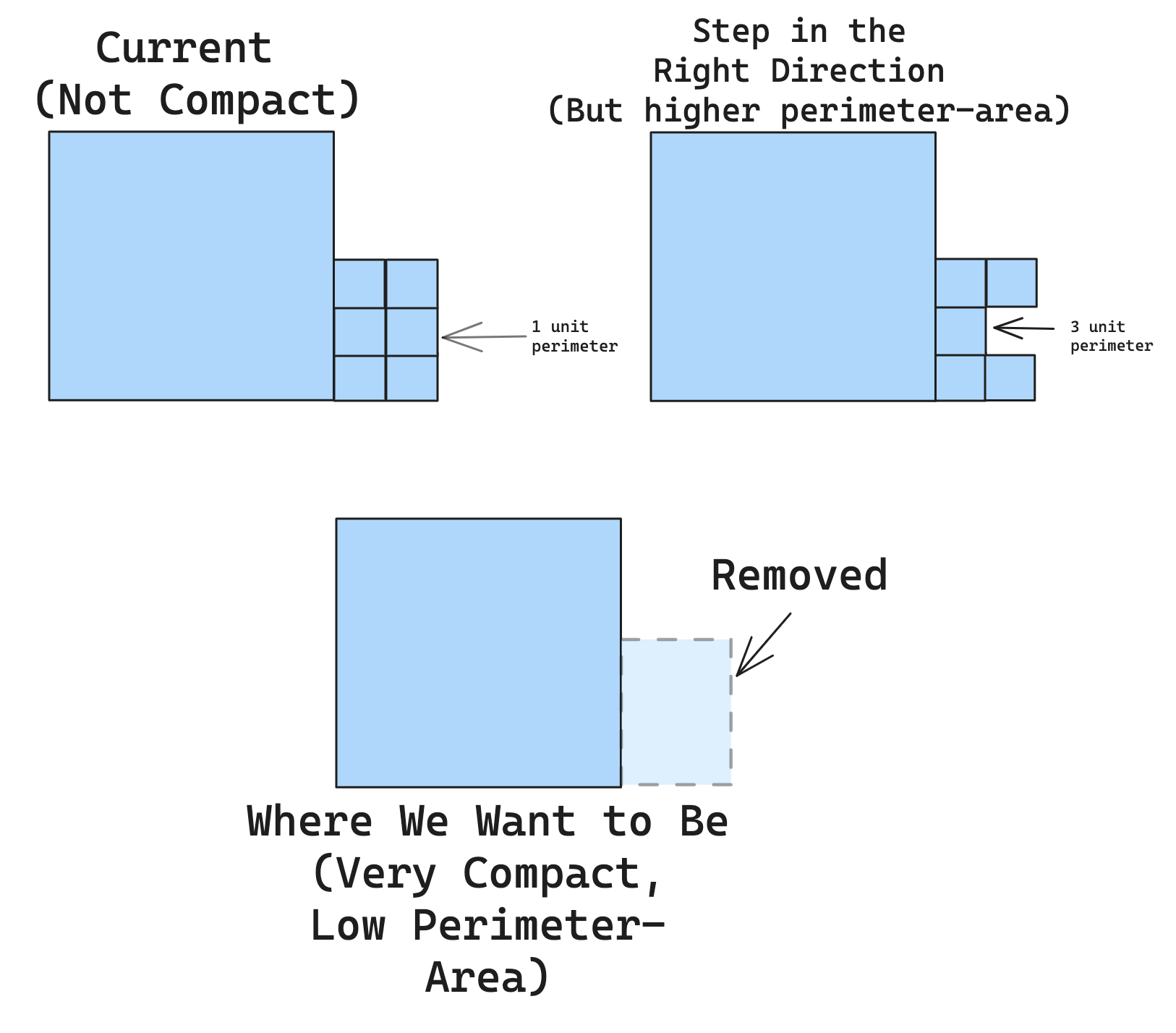
The perimeter-area ratio doesn’t do a good job of optimizing for compactness for a similar reason to why simulating an election doesn’t do a good job of optimizing for partisan bias. The perimeter-area ratio is non-monotonic, meaning that it’s not always decreasing as we move towards more compact districts - instead, it might increase before decreasing (remember smaller is better) when we move towards the most compact shape. This means that our simulated annealing algorithm again can’t measure small step-by-step progress - even if it’s moving in the right direction, our evaluation function might tell the algorithm that the new solution is worse!


An alternative way to optimize for compactness is to instead try to reduce the average distance of each tile from the center of mass of the district. This favors changes removing extremities in a district because they will have a dramatically higher distance from the center. It also is monotonous - taking a step towards increased compactness will always reduce the average distance between all tiles and the center of the district. I have not implemented this yet but this is something I would like to add to this project.
Additionally, the target margins of victory are chosen by the human. It’s fairly easy to choose numbers that pack, but it would be interesting to find the best margins of victory that might lead to needing fewer packing districts.
The weights in the evaluation function could also be tuned - because the evaluation function is a weighted sum, the algorithm will heavily prioritize characteristics with a higher weight. Something like a grid search of parameters might be possible to choose better coefficients, although the ones I have choosen do a decent job balancing population with partisan bias.

Code

View the full project here. This article was focused on gerrymander.py