Mini-RCNN Pt. 1 - What is Object Detection and how do RCNN models do it?
What is Object Detection
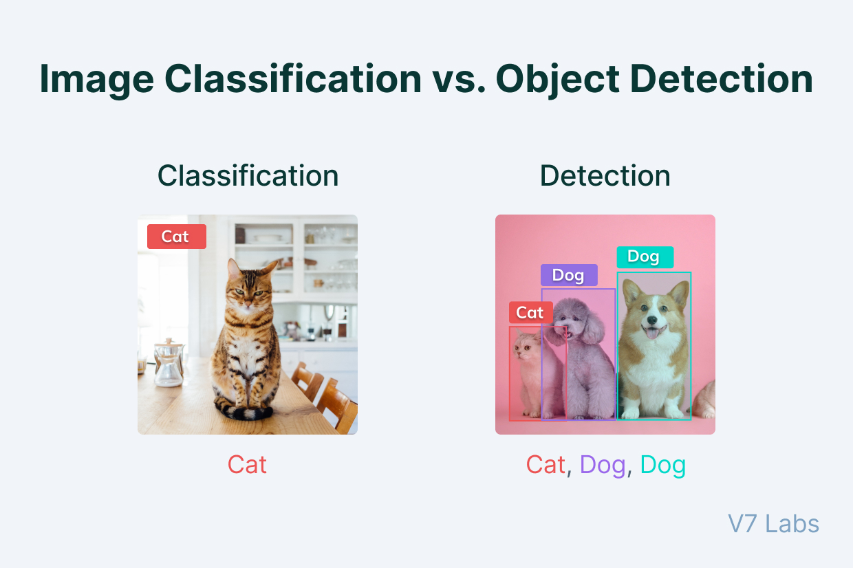
You probably know what image classification is - a model takes an image with some kind of object and labels what the object is. Object Detection is slightly more complex. Instead of an image with only one object, object detectors have to deal with images with multiple objects, separately labeling what each object is. Object detectors also have to localize each object, drawing a bounding box around each object.
Intro + Why RCNN?
Recently I’ve been working on finetuning YOLOv8 for a paper I’m hoping to submit for ISEF. YOLOv8 comes bundled up with the Ultralytics package, so finetuning and inference can be done without knowing anything about the model architecture, but I was nonetheless curious about what was actually going on under the hood. YOLOv8, is of course, just one model architecture that can be applied to Object Detection - RCNN, Fast/Faster RCNN, and SSD models fill similar roles.
YOLO stands for You Only Look Once, and it offers excellent performance at real-time speeds. “You Only Look Once” means that an image only passes through one neural network, so it’s much faster than two-stage detectors like RCNN and Faster RCNN.
I thought that actually implementing an object detector (nearly) from scratch would be an interesting side project, but after spending quite a bit of time reading and rereading the original YOLO paper, I decided that the YOLO model was just too difficult for me to implement from scratch. The YOLO model is actually quite hard to understand conceptually, because it needs to perform the same task as a two-stage detector with only one step. Instead, I’m choosing to implement RCNN, which was first proposed 2013. Fast/Faster-RCNN are both later improvements on the original RCNN architecture, but they all use a 2-stage process and are therefore slower than YOLO and SSD.
However, I actually think that RCNN is a more interesting model to implement from scratch - they use some really cool algorithms like Greedy Algorithms/Selective Search and Support Vector Machines.
Sliding Window Models - Leading up to the RCNN
While image classification and object detection are two different tasks, they do share clear similarities. Your first thought might therefore be to apply image classification models to object detection. Since classification models can’t draw bounding boxes or label multiple objects, we’ll need to use an algorithm called sliding window search. I like to think of sliding window search as being similar to a convolution operation, but with a classifier model taking in an image of dimensions NxM replacing the N x N kernel. We run the image classifier model on each N x M “window” of the image, using the N x M window as the bounding box if an object is detected. This window slides across the image by some step size so that the entire image can be processed.
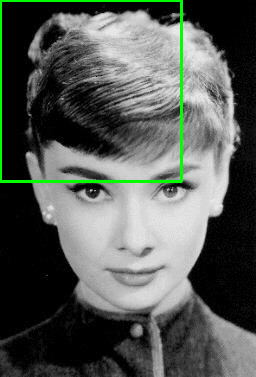
In the example above, a classifier for eyes, noses, and lips can be run on each window, which eventually “slides” over those objects. Every time the classifier labels an eye, nose, or lip in a window, we save the position of the window and the label from the classifier.
Sliding window models are indeed somewhat capable and were the SOTA in the early 2000s, with models such as Viola Jones Detectors being used to detect human faces.
Problems with Slinding Window Detectors
However, sliding window detectors suffered from several problems - chief among them the inflexible window sizes. In the real world, objecs have diverse aspect ratios - a human and a car don’t have the same aspect ratio, and therefore can’t both be effectively captured by the same window size. Additionally, large window sizes can introduce the possibility of multiple objects we want to detect being in the same window, confusing our classifer which was designed to only label individual objects. The solution is then to slide multiple windows across the image - we would need to slide windows of different sizes, along with windows of different aspect ratios for each size (these sizes and aspect ratios are often determined by a human for every single object class). We would then need some sort of way to remove duplicate detections from our many, many sliding windows which will overlap with each other. That means that hundreds of thousands or often millions of windows must be classified - an exhaustive search is performed for every possible position of every window on the image. That’s why the peak of sliding window detectors was in the early 2000s, when fast algorithms like SVMs and random forest classifiers along with hand-coded image features were still the primary methods used for image classification - running a more performant but slower CNN would be completely infeasible on so many samples. Of course, sliding window detectors are still a reasonable solution if there are very few object classes - fewer object classes means fewer aspect ratios for windows.
The RCNN
The RCNN, standing for Region-based Convolutional Neural Network, sought to address the speed and aspect ratio problems of sliding window detectors, while also harnessing the power of CNNs over simpler classifiers.
Instead of sliding windows of different sizes over every possible region, RCNN uses a region proposal algorithm to generate windows of the full image. The region proposal algorithm generates several hundred to a few thousand region proposals of various sizes which are far more likely to closely match the bounding box of an object than the vast majority of possibilities sliding window detectors need to process. A CNN is then used to compute each region’s features, which are fed into a SVM image classifier. You can think of the region proposal stage as generating possible bounding boxes (regions of interest) and the classification stage as filtering and labeling the possible bounding boxes. RCNNs offered a massive performance improvement over sliding window detectors because their region proposal stage allowed slower CNNs to be applied to the relatively fewer windows (around 1000 compared to potential millions for sliding window detection).
Of course, RCNNs have their own issues. Most of the region proposal algorithms aren’t trained on a dataset in conjunction with the CNN and the SVM, so region proposals are generally far from perfect. The most popular region proposal algorithms also generate a lot of region proposals - although 2000 is a lot better than the number of windows from sliding window detectors, RCNNs can’t even come close to real-time detection. Additionally, the final SVM classifier, although fast, is not ideal - we’d much prefer to just use a NN for classification. The entire model is also obviously not differentiable. These issues are all solved in clever ways in Fast-RCNN and Faster-RCNN, but I really like the conceptual simplicity of RCNNs and their use of 3 different algorithms.

RCNN Region Proposal: Edge Boxes and Selective Search
All region proposal algorithms need to return a list of windows that are likely to contain objects. Of course, region proposal algorithms are not perfect, so they have to balance between precision and recall like any other model (where a true positive is if a proposed window actually contains an object). Precision is equal to the algorithm’s True Positives/(True Positives + False Positives) or How Many Were Correctly Labeled Positive/How Many Were Labeled Positive. You can think of precision like quality - a region proposal algorithm with a very high precision is very unlikely to return irrelevant regions, although it may miss some relevant regions. Recall is equal to the algorithm’s True Positives/(True Positives + False Negatives), or How Many Were Correctly Labeled Positive/How Many Actually Are Positive. You can think of recall like quantity - a region proposal algorithm with a very high recall is likely to not miss any relevant regions but may also return some irrelevant regions. For region proposal algorithms, we want to select algorithms and parameters that lead to a high recall - we’re willing to waste some time checking irrelevant regions if that ensures that we won’t miss any relevant regions.
Region proposal algorithms can be evaluated by themselves by computing the recall between the proposed regions of interest to the actual bounding boxes of a dataset, with the labels being ignored. Remember, we just need the region proposal algorithm to do a good job drawing boxes around possible objects.
2 of the most fastest and best performing algorithms for region proposal are selective search and edge boxes. Although, these hard-coded region proposal algorithms are replaced with a learned region proposal network in the SOTA Faster-RCNN models, they are still quite interesting in how they do a decent job on a difficult task using a combination of simpler algorithms. They’re also nice in how they are dataset agnostic - edge boxes and selective search can do a good job proposing regions of interest regardless of whether they’ve seen a particular object before.
Edge Boxes:
Edge boxes are one of the most intuitive region proposal algorithms and also offer excellent performance. Given 1000 proposals, edge boxes achieve 96% recall @ IOU=50 in just 0.25 seconds on the Pascal VOC dataset. However, I couldn’t find a ton of resources on it unlike the more popular selective search, so I’ll do my best to condense the actual paper published by Microsoft Research in 2014 here.
The edge box method seeks to use the edges of an image along with the contours they form to draw regions of interest, since contours generally represent the boundaries of objects. A contour is a set of connected edges forming a closed loop.
The edge box algorithm starts in much the same way as a sliding window detector by sliding windows of varying sizes and aspect ratios across an image. However, instead of running a slow classification model, the edge box algorithm only needs to return a score for how likely the window is to contain an object. This method doesn’t suffer from the same speed and performance issues of sliding window detectors because it runs a very fast algorithm to score each box. It then only returns a certain amount of the top scoring boxes, which can then be fed to the second stage, which is a high performance CNN in a RCNN model. By using this scoring/cutoff process, edge boxes save a lot of time in the comparatively slow classification stage.
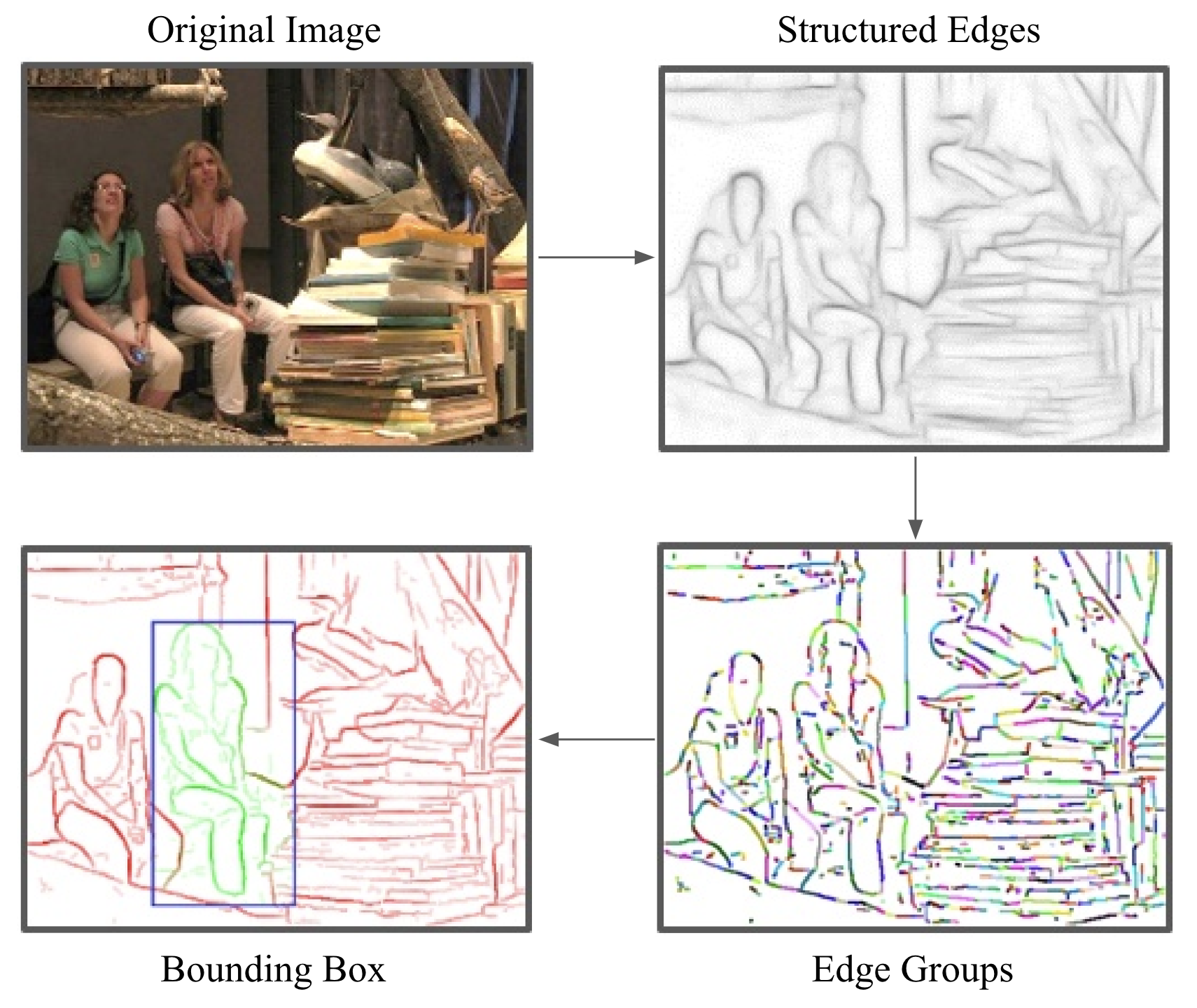
To start,
An edge map is generated using the OpenCV Structured Edges detector (I may not implement this from scratch depending on how much time I have). An edge map is a bitmap containing the edge magnitudes and edge orientations/normals (direction of changing gradient in the image that results in an edge). To thin edges (which may be multiple pixels wide) and deal with noise, we use Non-Maximal Suppression along the edge normals (I will cover this more in later posts) and remove ignore any edges with magnitude < 0.1. These steps results in Image 1 in the example above.
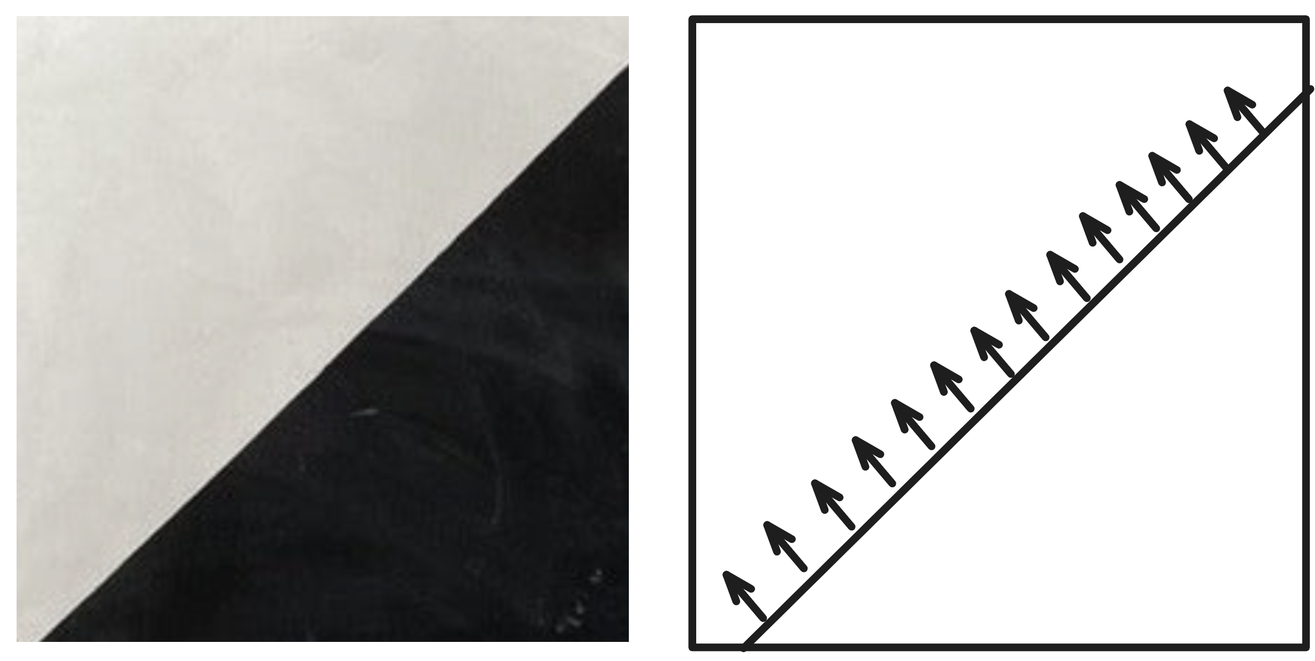
Edge groups are then computed by repeatedly combining 8 edge pixels until the sum of their orientation differences is greater than pi/2 rad (Image 3 in the example above). We store the mean position and mean orientation of each edge group.
We then run the sliding window search, scoring each window with the following steps: