Algorithmic Gerrymandering Pt. 1: Modelling population and voter distributions
What is Gerrymandering?
In a representative democracy, a state is divided into districts. Each district can elect one representative. States redraw districts every 10 years following the census - regular redistricting is important to ensure that districts are representative of a state’s changing demographics. The winner of each district is decided by the plurality rule (candidate with most votes wins), making each individual district winner-takes-all.
- Congressional Districts: States are divided into congressional districts based on the number of representatives they get in the US House of Representatives. NC, which has 13 house representatives, is divided into 13 congressional districts. Congressional Districts must have (nearly) equal populations.
- State House Districts: States are divided into districts for choosing state level representatives. The NC House of Representatives (distinct from the US House of Representatives) has 120 members, chosen by 120 individual districts. State level districts are allowed to have larger deviations in population than congressional districts.
- State Senate Districts Similar to house districts, states are divided into senate districts to choose state senators (distinct from US Senators). The NC Senate has has 50 members, chosen by 50 individual districts.
In theory, the total body of the elected representatives should, as John Adams put it, be an “exact portrait, a miniature” of the people as a whole - a 60% blue state should have 30 blue US senators (out of 50). The representatives should also match the demographics of a state - a 20% Asian state should have 10 senators (out of 50) supported by Asians. To achieve this, districts should be balanced - with some majority red districts, some majority blue districts, and districts with a majority from a particular demographic.
However, through gerrymandering, partisan mapmakers can create district maps which favor one party, regardless of the actual voter preference.
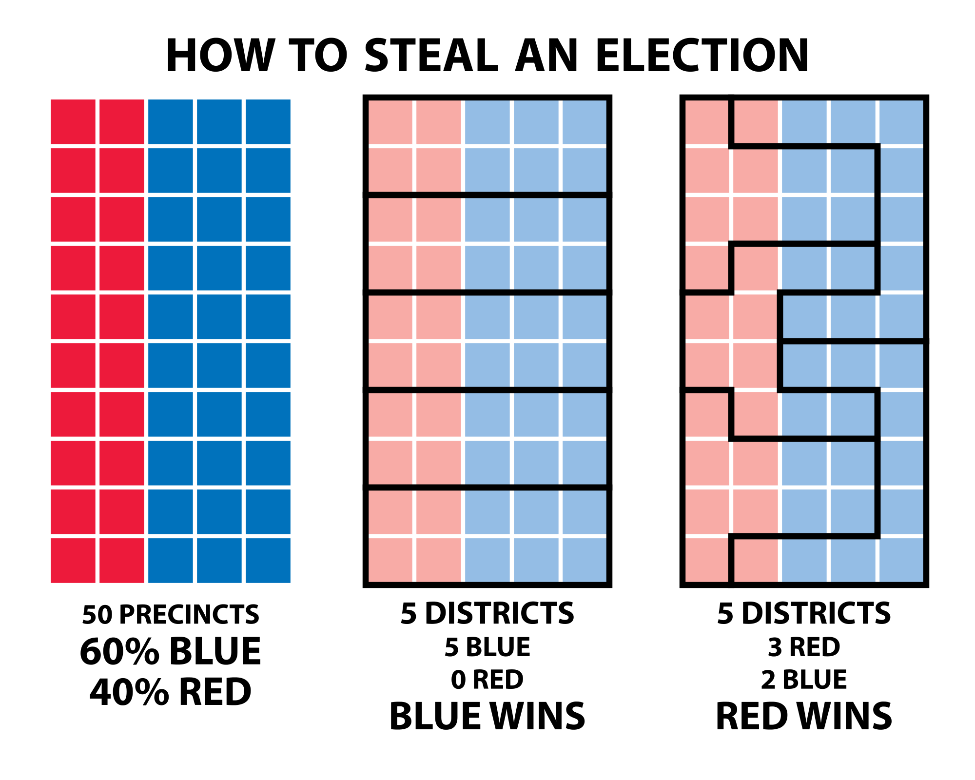 In the image, an ideal districting should make 2 red districts and 3 blue districts to fairly represent all voters (40% red, 60% blue), but by cleverly dividing the region into districts, we can have 5 blue districts (100% blue) or 3 red districts and 2 blue districts (60% red).
The two main methods of gerrymandering are cracking and packing. Cracking splits a voting group into many districts, giving them a local minority in each district, regardless of their actual share of the population. Since each district is winner-takes-all, cracking can completetly wipe out a minority’s voice: 49% of the vote in 5 districts is still 0 representatives. This is demonstrated by the 1st districting in the image, where red voters have a local minority in every single district and therefore have no seats, even though they make up 40% of the population.
Packing involves concentrating most of one group’s population in a few districts, so that the group has less representation in every other district. Since margin of victory doesn’t matter in a district, the extra voters in a packed district make no difference in the result - their vote is “wasted”. This is seen in the 2nd districting, where most of blue’s voters are packed into the 2 rightmost districts, which they win by an overwhelming majority, but at the cost of losing the other 3 districts.
State population and voter preference distribution in the real world
Instead of taking census and polling data from real states, we’ll be trying to gerrymander a lattice model, like the grid we saw in the example above. However, the example was missing two important features: it assumed that the population of each tile was equal, and that each tile was either completely red or completely blue. The population aspect of each tile is critical because a tile with more population has more impact on a districts vote - a district made up of a red tile with 9900 voters and a blue tile of 100 voters is not 50-50, its 99% red. A gradient of voter preference is also important - some geographic regions are more moderate than others.
Population
Although we’re generating our own model, we still want it to be as accurate as possible, so the population distribution should follow patterns in real states.
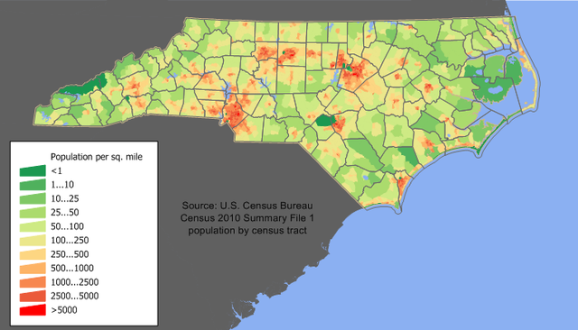
Looking at a population map of NC, population is concentrated around a few “spikes”, and gradually falls off from there, forming a smooth gradient. Aside from the population centers and their immediate surroundings, most of the state has a relatively low population.
Voter Preference
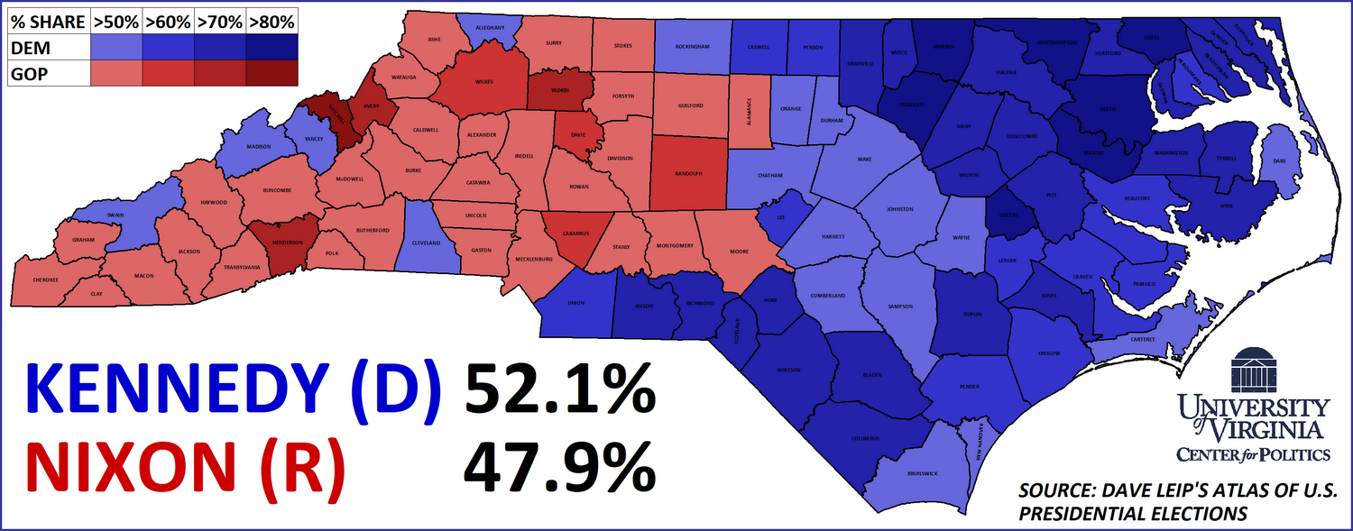
As for voter preference, we see a that each party has its most extreme hotspots, and voters become more moderate as they move away from the hotspots. Interestingly, the most moderate voters are the ones between radical red and radical blue hotspots.
Implementing the lattice model
Recall that a lattice model is a grid representing an area with each tile representing a subdivision of that area (maybe a square mile or a precinct). Each tile has a voter preference (a gradient between red and blue) and a population. To make the coding a little easier, -1 will be the most extreme blue partisanship and 1 will be the most extreme red partisanship, with 0 representing an area with no political affiliation. To translate into percentages, 1 is 100% red, 0.2 is 60-40 red, 0 is 50-50, -0.2 is 40-60 red, etc. In other words, the decimal is the difference between the red percentage and blue percentage. The population of the entire model is the sum of the population of each tile, and the overall political preference will be the sum of the partisanship of each tile multiplied by its population divided by the total population.
Assigning populations
To replicate the population spikes we saw in a real population map, we’ll randomly assign a few tiles to be our population centers and give them a large population. Every other tile will start with a population of 0. Then, we give every person in these population centers a random number of moves based on a Gaussian distribution centered around the number of moves it would take to get from the center of the grid to a corner. Then, we let each agent randomly makes moves in one of the 4 cardinal directions until it has expended all of its moves, and add one to the population of the tile it ends up on. Because a) going far from the population center is more unlikely because it requires many moves in one direction in a row and b) most agents don’t have enough moves to go very far from their starting point, most of the agents remain concentrated at the population center or in its immediate vincinity. However, this method does give us some random noise each time, so we aren’t constantly generating the same population spread.
Assigning voter preferences
We saw that voter preferences formed a gradient between the most extreme source points, and that the region in the middle was the most moderate. The closer a region is to a radical hotspot, the more radical it is. A region perfectly in between to radical areas is relatively neutral - suggesting that 2 radical regions can cancel each other out. To replicate this, we randomly assign some tiles to be extreme areas with a voter preference of 1 or -1. Every other tile has a voter preference of 0. We then have each extreme tile add its voter preference divided by d (+-1/d) to every other non-extreme tile, where d is the distances from the extreme tile to the other tile. This ensures that closer extreme tiles have more influence, and also creates the smooth gradient - a tile in the middle of 2 extreme tiles will have preference +1/d - 1/d = 0.
Combining these methods, we can generate a lattice model that looks like this:
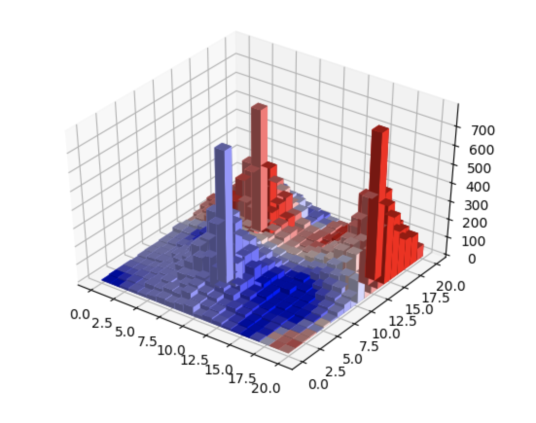 The example created is a 20x20 lattice model with 3 population source points - we have a smooth fall off of population around the 3 population centers and a gradient between radical regions with more moderate tiles.
Next, to create a gerrymandered set of districts for our lattice model, we’ll have to assign each of these tiles to a district in a way where the total political preference of most districts (the sum of all the voter preferences of the tiles in the district) slightly favors the favored party.
The example created is a 20x20 lattice model with 3 population source points - we have a smooth fall off of population around the 3 population centers and a gradient between radical regions with more moderate tiles.
Next, to create a gerrymandered set of districts for our lattice model, we’ll have to assign each of these tiles to a district in a way where the total political preference of most districts (the sum of all the voter preferences of the tiles in the district) slightly favors the favored party.
Code
The full source code for generating and viewing the population map can be found here